
Google Sheets is used by numerous people all around the globe as a reliable tool for data entry. No matter personal or official, one can create, edit and collaborate with others on spreadsheets from supported gadgets with the Google Sheets. You might have used the Google Sheets to get your work done. However, there might be a case when duplicates in Google Sheets entries ruin your whole venture. In case if you’re looking for nifty workarounds to fix the nuisance with the duplicates, let’s see how can it be avoided.
Thankfully, Google Sheets features some indirect mechanisms to eliminate the duplicates. Here, we’d be going through some of them.
Guide to Remove duplicates in Google Sheets
Using the Addon – Duplicate Remover
Google Sheets support a plethora of Add-Ons which can be installed based on your need and purpose. For removing Duplicates, Google Sheets has an add-on called Duplicate Remover. Using the add-on we can remove duplicates with few 3-4 steps.
- On Google Sheets, go to Tools>>Get the add-on
- Enter duplicate on the search bar to see all the available tools with duplicate as a keyword
- From the available options, choose Duplicate Remover from Adlebit
Once installed, Duplicate Remover will be featured on the Google Sheets. So, in order to remove duplicates, Go again to Tools and choose the add-on, Remove Duplicates.
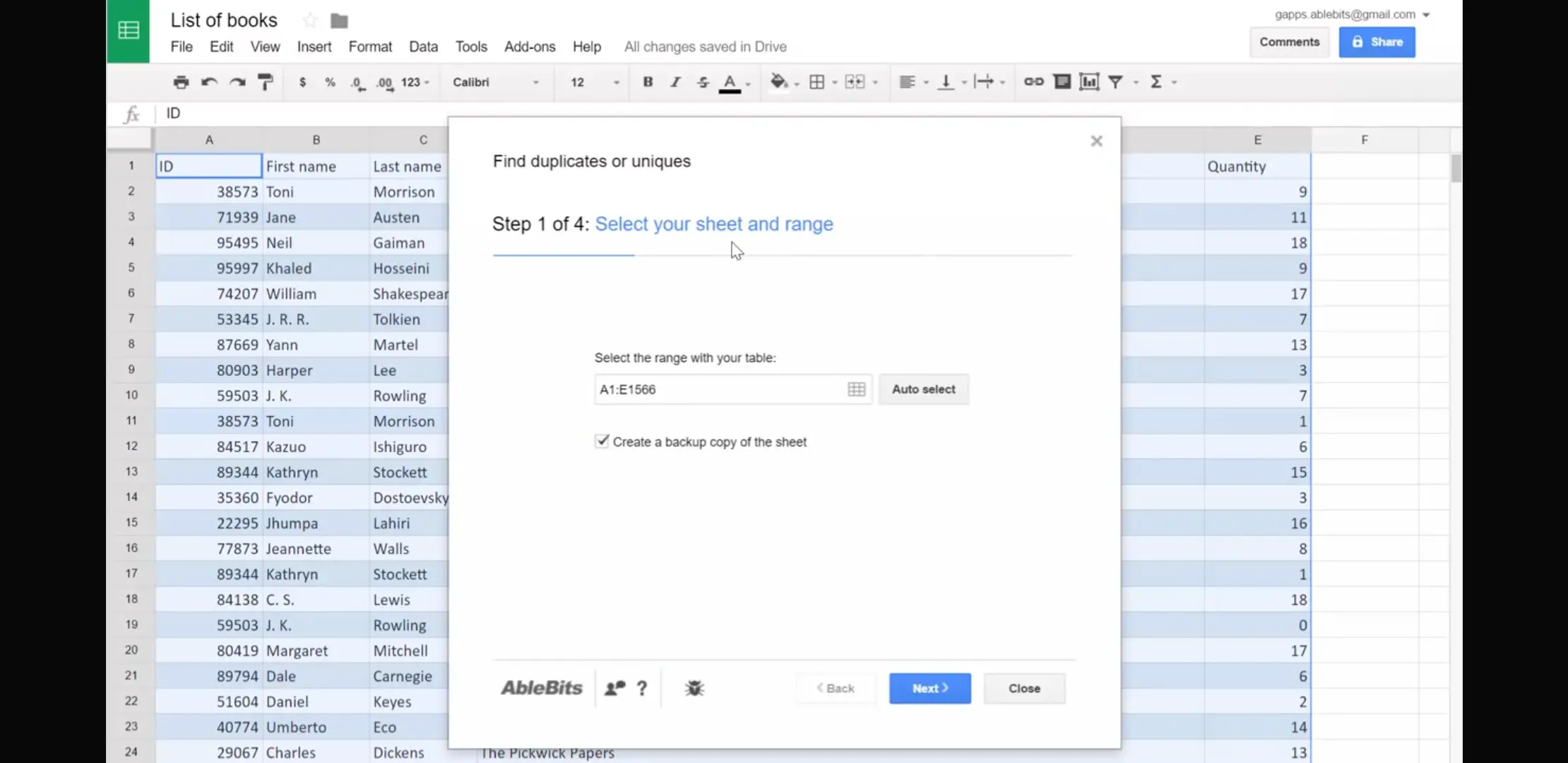
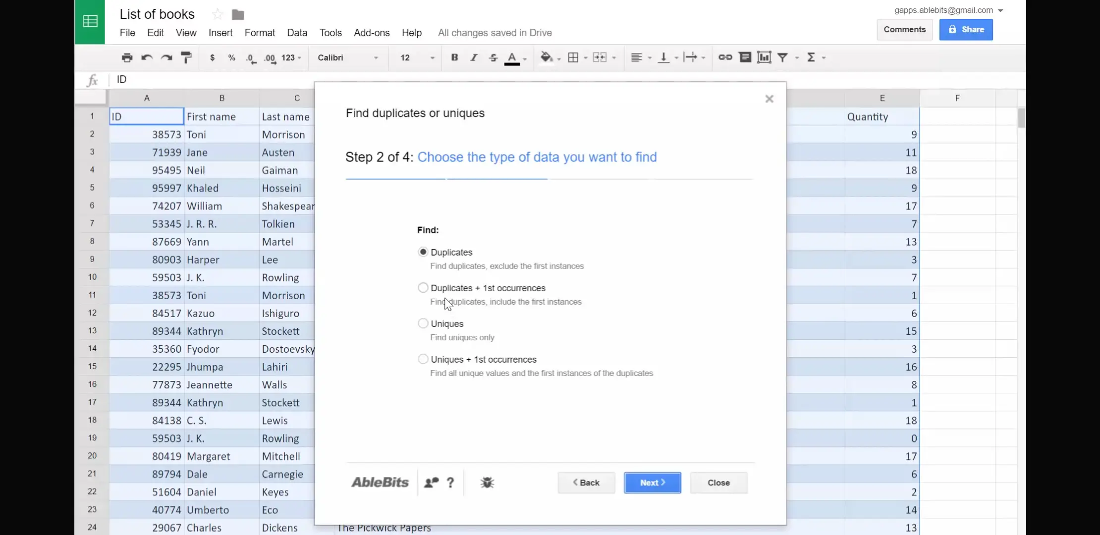
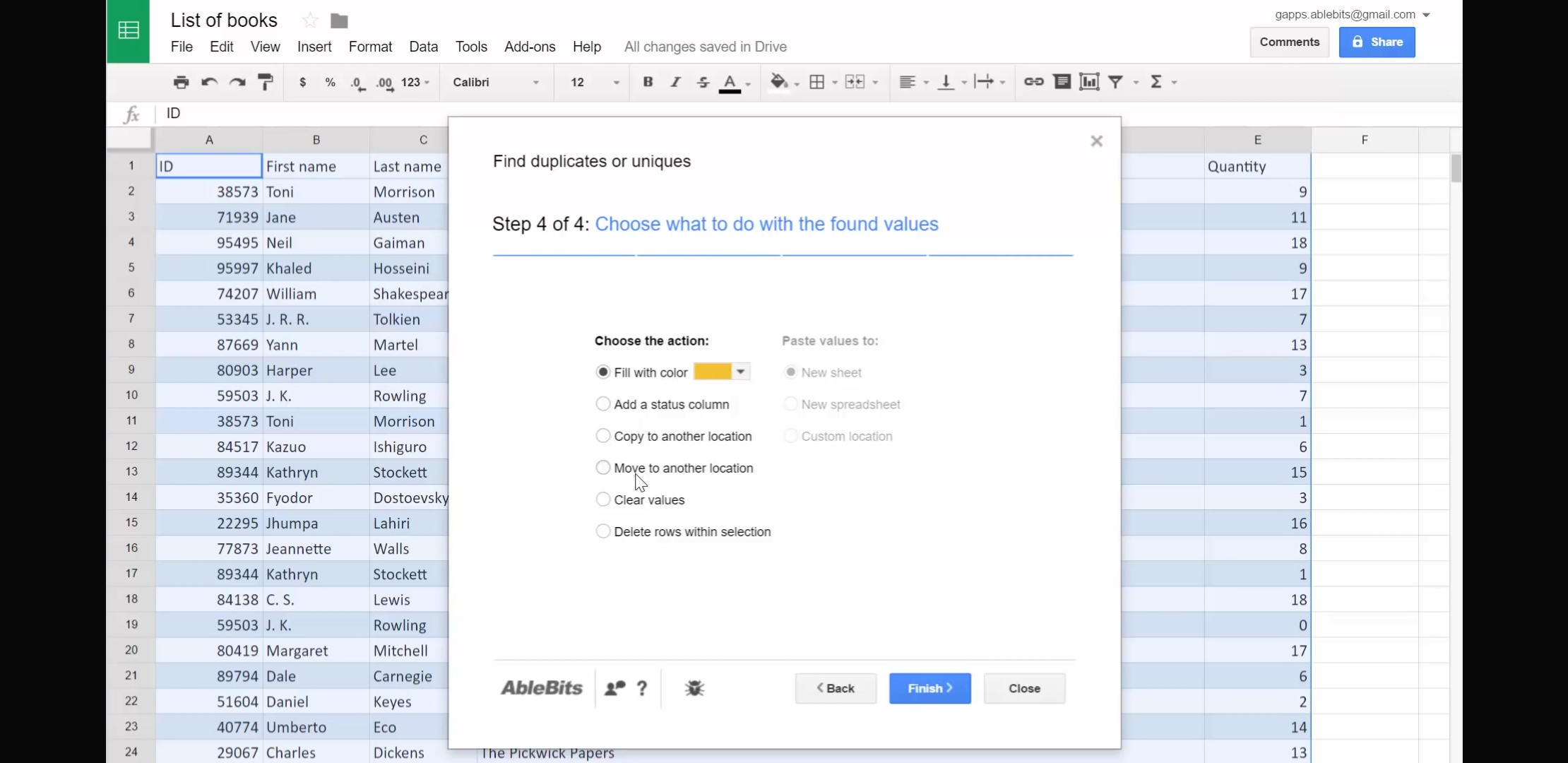
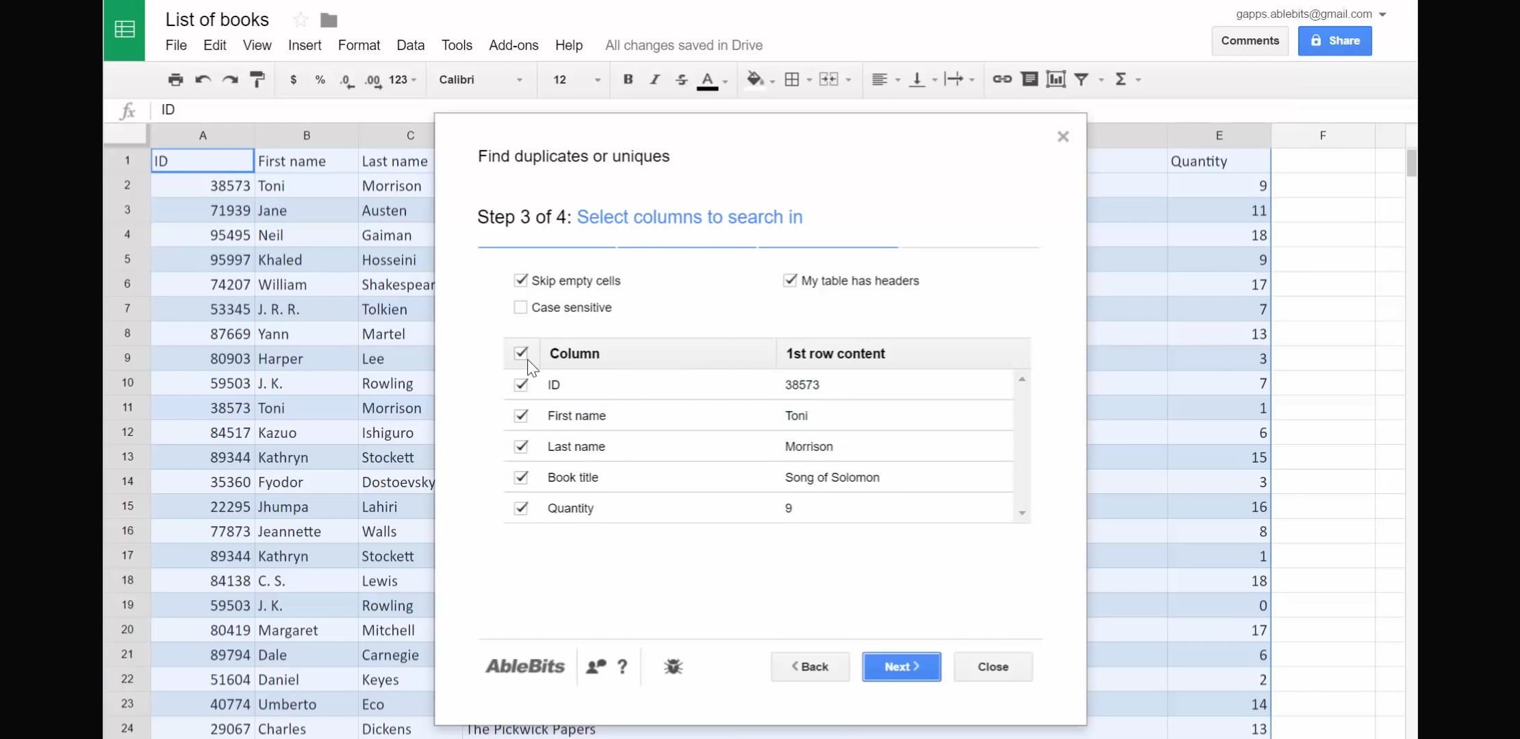
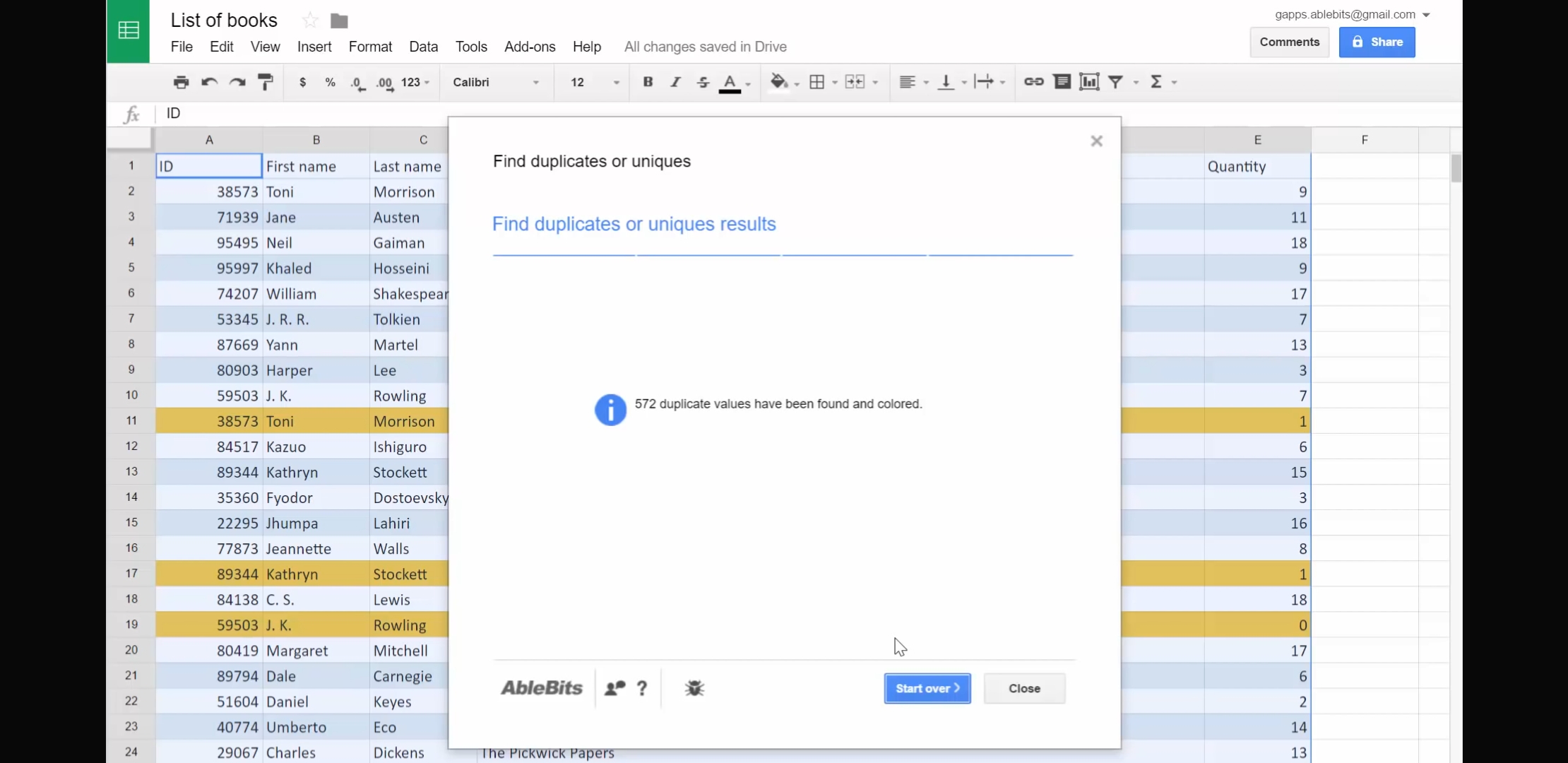
The add-on will take you to 3-4 series of steps to get your preference. Moreover, options such as whether you want to highlight duplicates, delete them, create a new copy of your data and such are available.
Also read:Best Google Chrome Tab Managers
2. Conditional Formatting
In order to remove duplicates using conditional formatting, we need to go through two steps. The numero uno is to highlight the duplicates, and then to remove the highlighted contents.
- Highlight the duplicates
- Remove the highlights
First of all, we can highlight the duplicates, for that select your dataset and open the conditional formatting sidebar (under the Format menu).
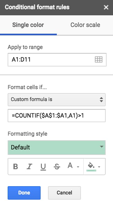
- Under the “Format cells if…” option, choose custom formula is (the last option) and enter the following formula.
=COUNTIF($A$1:$A1,A1)>1 (This formula checks for duplicates in column A).
The duplicates in column A will be highlighted on your data set.
- In case you want to highlight the whole row, then change the above code a little by adding $ sign before the last A1.
=COUNTIF($A$1:$A1,$A1)>1
3. Using Pivot Tables
Pivot Tables are useful especially for exploratory data analysis. Pivot Tables can be used to search for duplicates in Google Sheets. They’re flexible and fast to use, also helps to phase out any duplicates in your data.
- Highlight your dataset and create a Pivot Table (under the Data menu).
- A new tab opens with the Pivot Table editor.
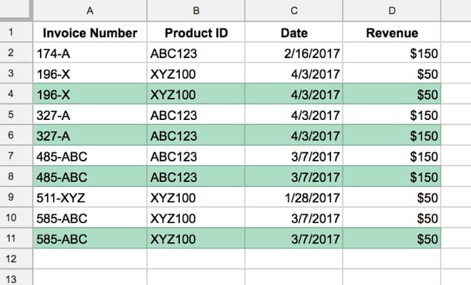
- Under ROWS, choose the column you want to check for duplicates (e.g. invoice number). Then in VALUES, choose another column (I often use the same one) and make sure it’s set to summarize by COUNT or COUNTA (if your column contains text), like this:
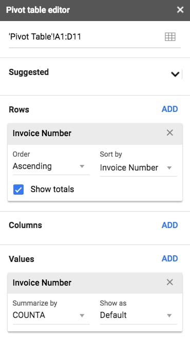
You can see that duplicates values (for example 196-X) will have a count greater than 1. From here you can look up these duplicate values in your original dataset and decide how to proceed.
Also Read: How to disable Google Assistant on Android and iOS
Apart from the above mentioned three methods to remove duplicates, there do exist some other method such as by App Script. However, these are the simplest method which you can use to phase out the duplicates.